River Discharge Function
Below is an analyses of river discharge using data relative to the Salt River and Tempe Town Lake. The images below depict the various variables pertaining to the river discharge function and their relationships to one another. For each comparison, the variables not in mention are held at a constant value for accuracy.
To start, here is the Matlab script used to compute the variables and values that make up the plots below. These values include river velocity, discharge, channel roughness, channel radius, depth, slope, and width.
River Discharge Matlab script
The first figure is a plot that shows the relationship between the velocity of the river water and the channel slope of the river varying about 12 degrees.
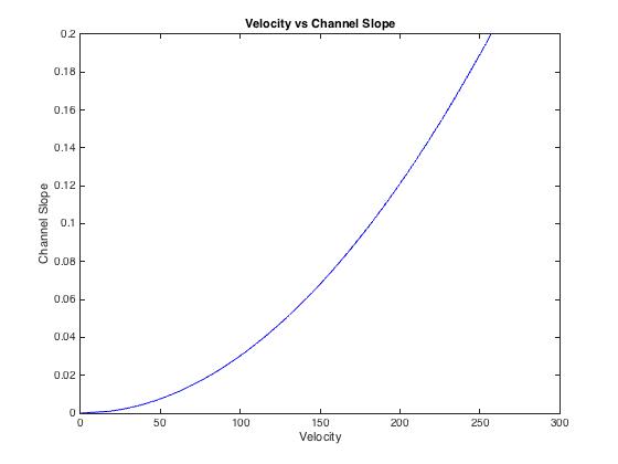
As you can see in the plot, as the slope of the channel increases, so does the velocity. Basing that on basic gravitational physics, that result makes total sense.
Next, I plotted river discharge against the channel slope, using the same 12 degree variance.
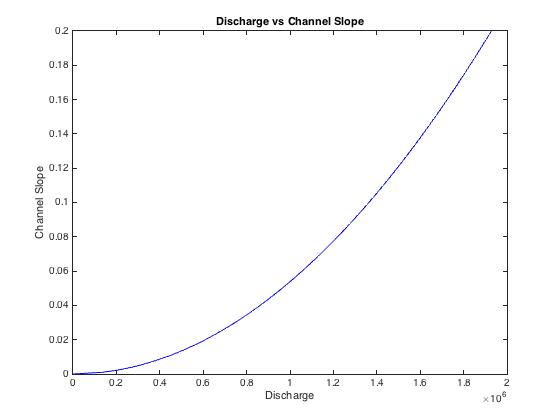
Much like the previous plot, as the slope increases so does the discharge levels. This is also due to gravitational forces.
We know now how velocity and discharge are related to the slope of a river channel, so now we will look at the relationship between velocity and the hydraulic radius of the river, which is calculated using the depth, width, and the wetted perimeter variables.
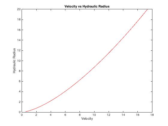
The graphic here shows that with increasing hydraulic radius, the velocity also increases. So, the bigger the river channel, the greater the river velocity as long as all other variables are held constant.
Continuing on the trend of examining river velocity, the next relationship to be examined is between river channel velocity and the roughness of the channel surface. For the roughness values, I used the Manning roughness coefficient ranging from a smooth almost glasslike surface to a rough mountain stream surface.
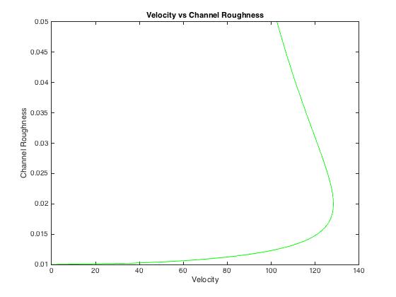
The velocity of the river channel dramatically increases at first when the channel roughness is smooth, but eventually reaches a point where the roughness of the channel counteracts the flow of the river and begins to slow the velocity the more rough it gets.
Lastly, we examine the relationship between river discharge and the roughness of the river channel surface.
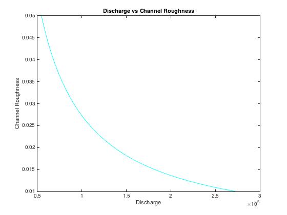
This plot begins with the mountain stream roughness value and shows that river discharge is at its weakest value at this point but then as the roughness subsides and becomes smoother, the discharge gradually increases as well.
To go along with the data analyses above, the problem given to us is with river values being 19 feet deep, 850 feet wide, roughness being estimated, and the slope being 0.0013, find the probable velocity and discharge of the river at this point. I gave a roughness value of 4 since even near Tempe Town Lake, there is still plenty of uneven river bottom surface and vegetation. By using the Matlab script (link at the top of the page), I implemented these values which resulted as such;
width = 850.0 feet and depth = 19.0 feet
Wetted Perimeter = 888.0 feet and R = 18.2 feet
velocity = 9.3 feet/sec
discharge = 150006.5 cubic feet/sec
Finally, given a similar problem set but with values being 900 feet wide, and 40 feet deep, using the Matlab script once more I calculated these values using the same roughness justification as the problem before;
width = 900.0 feet and depth = 40.0 feet
Wetted Perimeter = 980.0 feet and R = 36.7 feet
velocity = 14.8 feet/sec
discharge = 534299.5 cubic feet/sec
If back in 1993 the Salt River flowed at 100,000 cubic feet per second, and my calculations are relatively accurate, that would mean that back in 1993 the river was not at a bankfull flow, since the calculation shows that the discharge could reach more than 5 times that amount at the max width and height of the river.